|
LBIBCell
|
|
LBIBCell
|
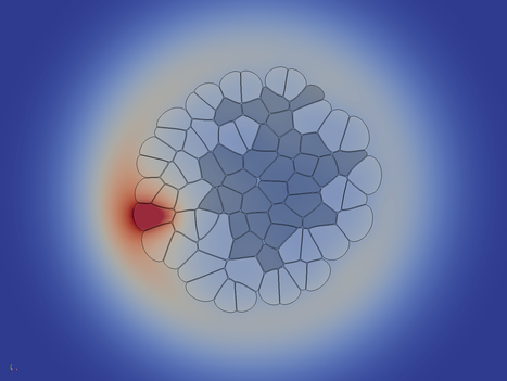
In the following example, a few fundamental biological processes are implemented: cell growth and division, differentiation, and the secretion and diffusion of a single biochemical molecule.
The initial configuration consists of one single circular cell of type 1 in the middle of the domain. Type one cells grow and divide at a high rate, so the first cell soon divides multiple times. The division is triggered when a certain threshold cell area is exceeded. The cell division plane is chosen to be perpendicular to the longest axis of the cell (random direction is implemented as well).
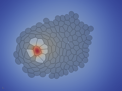
The first (and only the first) cell secrets a molecule S which is allowed to freely diffuse across the tissue, where it is degraded slowly. The cells integrate the concentration S over their area. Whenever the concentration falls below a threshold value, the cell is differentiation into the cell type 2. This cell type does not grow and proliferate any more: the cell area is kept constant.
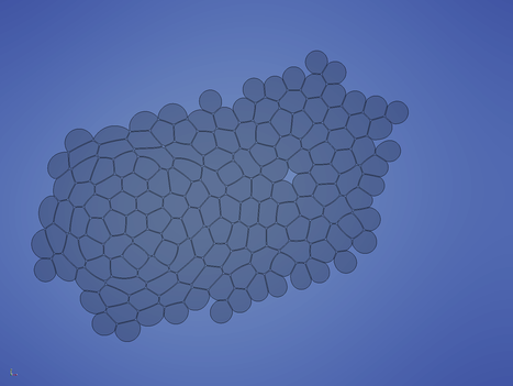
After a while (5000 time steps in this case), the inital cell ceases to secret the differentiation-inhibiting molecule, and soon after all cells differentiate.
In the last phase of the simulation, the cells start to rearrange locally to relax tensions. The simulation can - in priniple - continued until steady state is reached.
In the following sections, the setup, input and output of the simulation are discussed in detail.
The most important, global simulation paramters are read from a file /apps/config/tutorial_01_parameters.txt:
CurrentIterations is the time step to start from. We start from zero. Iterations denotes the number of time step to be executed in this simulation. ReportStep tells how often to save simulation results to files. Here, every 10th time step. Next, the size of the simulation domain is given, followed by tauFluid, which is the Lattice Boltzmann relaxation time of the fluid solver. This parameter is directly related to kinematic viscosity of the fluid (The numerical background and the formula can be found in the publication). Under CDESolvers, the user-crafted CDE solvers have to listed. Make sure that you always pass 2-tuples, consisting of the CDE solver name and the corresponding Lattice Boltzmann relaxation time (which is directly related to the diffusion coefficient; please consult the publication).
The input geometry can easily and intuitively be generated by custom matlab or python scripts (or even by hand). The matlab script /apps/config/config_circularcell, for instance, can be used to generate a single round cell. Let us have a look how the file is structured:
Under the first header #Nodes, all the geometry points are listed. The first number is the unique identifier which denotes that point. The identifier can be given freely (in any order), but it is in the responsibility of the user to make sure that no two points share the same identifier (this is not checked). Following the identifier, the x and y coordinates of that point are given.
Under the second header #Connection, the connectivity information is given. In every line, two point identifier have to be given to create a connection between them, followed by a domain identifier. This identifier is a unique number for the individual cell, and can be assigned freely by the user (same here: it is in the user's responsibility to make sure that it is unique and consistent across all the connections forming one cell; violation might cause undesired behauviour and segfaults which are hard to track). If desired, the connection can be configured with different boundary conditions for the different diffusing species. That topic will be discussed in the Tutorial 2: Turing Pattern on Growing Tissue.
Since the refinement of the membrane is automatically done by the simulation, the initial geometry of a simple square cell with side length 2 centered around {10,10} can be manually written as simple as that:
Please note that the cell has to be closed (the last line), and the polygon defining the cell has to be strictly given in counter-clockwise order.
Alternatively, the input geometry can be read from a .vtm (a vtk multiblock) file. The detailed description and de-novo generation of this format exceeds the scope of this tutorial. In short, a vtkPolygon is used to store the polygons representing the cells, together with some attributes (cell type flag, cell identifier). To get detailed information about vtk, please consult http://www.vtk.org/.
If you already have .vtm files (e.g. from a previous run, where you used the simple .txt format to start), you can use them as input without loss of any data. Maybe you don't want to start from a single rectangular cell each time, and rather prefer to start from an already big (relaxed) tissue, then the vtk format is perfectly fine. How to choose between those formats is described in Source Code Description.
Because the description of the set-up of the reaction-diffusion-advection solver is quite lenghty, is shown here: The Reaction-Diffusion Solver.
The mass solvers are intended to be used for simple operations on the fluid density. This is (currently) only the boundary condition of the domain. On the boundary, an iso-pressure boundary condition is enforced, i.e. we have a free boundary condition for the velocity field. Typically, our cells grow (increase in mass) and push out the surrounding fluid. The mass solvers could be implemented as BioSolvers, but we wanted have a clear division between pure physical processes (such as the domain boundary condition) and biological processes. For a more detailed description of the mass solver which is used in this example, please visit MassSolverBoxOutlet.
It is almost impossible to offer functionality of every biological behaviour one could possibly think of. Therefore, our approach is different: we offer a framework, which easily allows the user to implement and add small custom modules. The procedure is quite simple: you have to inherit from a base class to comply to the interface, implement a few functions, and add add your new module by just adding one line of code in your application (as described in Detailed Description). The general process how to create a new BioSolver is described here: An Empty BioSolver.
Please consult the following documentations for detailed description of the respective BioSolver:
We need the following library headers to create a Geometry (stores the cell geometry), GeometryHandler (stores the geometry and the lattices and performs operations on them) and SimulationRunner (manages the execution of the simulation) object:
The following headers are needed to write the simulation outputs. This can be adjusted to your needs: if you don't want to output the fluid solver solutions, there is no need to include vtkFluidReporter.hpp. In LbmLib/include/reportHandler/, you can also find more Reporters (which, for instance, write simple .txt based files which can be loaded in Matlab), or you can add your own custom Reporters.
We also need a few standard header files:
Now, we start with the standard main function. Exceptions will be caught in the end. The fileName will be used later to configure the Reporters.
It is convenient to store all the output files in an output folder. Therefore, we create the folder and clear its content (in case that it is already existing and having content from a previous run):
The log facility Log is configured such that the log file is stored in the same output folder as the simulation results:
Next, we have to feed the global simulation paramter container (Parameters) with our input parameter file:
Now we slowly envoke the central objects to life. The Geometry object stores - nomen est omen - the geometry. The initial geometry can be provided either in a proprietary txt format or a vtk format (as described in Simulation Input). The GeometryHandler constructor takes an Geometry object:
The ReportHandler object houses all the different Reporters. It is configured with the frequency of writing output files, which was loaded into the Parameters object:
Now, the SimulationRunner object can be initialized. The constructors takes the GeometryHandler and the ReportHandler objects:
The following vtkCellReporter stores the cell geometries, together with the attributes CellType (and unsigned integer) and the cell identifier (a unique unsigend integer used to identify individual cells).
If desired, the vtkCellPNGReporter creates simple snapshots of the cell geometries and saves them as .png images:
The vtkForceReporter saves the forces (which act between each two points) together with attributes (force type flag):
If biochemical species (CDE = convection-diffusion) are present, the all concentrations can be saved using the vtkCDEReporter. A coarsening factor can be used to reduce the data size (since this Reporter creates the largest amount of data). A factor 4 means that every 4th point is saved in one spatial dimension. Thus, the output size is reduced by a factor of 16.
Similarly, the fluid density and velocity field can be saved using the vtkFluidReporter. The coarsening factor works in the same way as for the vtkCDEReporter. Please note, that all Reporters got the same fileName: in this case, all the results are written into the same vtk multiblock (.vtm) file.
Next, the fluid and CDE solvers are initialized. By default, the fluid density is uniformly set to one, and the fluid velocity field to zero (if a custom field is desired, it can be passed here). By implementing the CDE solver modules, the user has to provide the initSolver() method and may specify custom initial values.
If initial forces are provided by the user, they have to be put into the force.txt file, which is used to initialize the force solver:
The last configuration steps consist of adding the different custom solvers. The MassSolverBoxOutlet is a standard free boundary condition for the fluid: by specifying a pressure of one at the boundary, the fluid flows out of the simulation domain. The BioSolverXX are described in more detail in Mass- and BioSolver Modules.
Now we are ready to run the simulation:
If an exception was thrown, it will be catched here:
To get an idea, the run time of the example is about 50 minues on an Intel(R) Core(TM) i5-3570 CPU @ 3.40GHz using 4 cores if you execute all the Reporters, and about 30 minutes if you only store the cell geometries and attributes. Similar to the input (c.f. Simulation Input), the output can be chosen to be in the simple proprietary .txt format, or in vtk format (as done in our tutorial). If you execute all the above Reporters, the output data size amounts to about 7.5 GB. If you only store the cell geometries and attributes, the data is reduced to less than 1 GB. Additionally, in the tutorial we dump every 10 time steps (which leads to 1000 snapshots) - which is extremely much. This is good for making a movie, or investigating the small details of rearrangement. You might want to reduce the frequency by a factor 10 or even 100 - thus also reducing the data size.
For easy, fast and high quality rendering of the results, we use ParaView. Although it is not the right place to give an thourough introduction to ParaView here, we now suggest some steps.
Visualizing the cell type and the domain identifier:
File → Open, then choose all the .vtm files Apply ctrl+space, type Extract Block and choose the Extract Block filter DataSet 0 and hit Apply ctrl+space, type Triangulate, choose the Triangulate filter, and hit Apply Solid Color to cell_type or domain_identifier
Visualizing the forces:
Cells_* ctrl+space, type Extract Block and choose the Extract Block filter DataSet 1 and hit Apply ctrl+space, type Threshold, choose the Threshold filter, and hit Apply Minimum and Maximum accordingly
Visualizing the concentrations of the biochemical species:
Cells_* ctrl+space, type Extract Block and choose the Extract Block filter DataSet 2 and hit Apply Solid Color to tutorial_01_CDESolverD2Q5_SIGNAL Outline to Surface
Visualizing the fluid density and velocity field:
Cells_* ctrl+space, type Extract Block and choose the Extract Block filter DataSet 3 and hit Apply Solid Color to density Outline to Surface Solid Color to velocity ctrl+space, type Glyph and choose the Glyph filter The following images give you a foretast of how the results of Turial 1 look like:
 1.8.6
1.8.6 
