LBIBCell
 All Classes Functions Variables Friends Pages
Tutorial 2: Turing Pattern on Growing Tissue

Model Description

The following tutorial builds up on Tutorial 1, with a few modifications.

Let's mention first what we don't need any more: differentiation. We have only one cell type here. But we have a more complex signaling model, consisting of two components. The first component is a receptor which lives on the surface of the cells (e.g. the apical membranes of an epithelium). It is allowd to move (diffuse) at a low rate, but it cannot 'leave' a cell, i.e. no-flux boundary conditions apply to the membranes for the receptor. The second component is a ligand, which is allowd to freely diffuse (e.g. in the cavity adjacent to the apical side of epithelial cells). One ligand binds to two receptor, forming a complex, and triggers biological activity. Therefore, we call the complex SIGNAL. The activity is cell growth and difision in our case: if the signal exceeds a threshold value, the cells proliferate at a high rate.

When we write down the non-dimensional signaling equations, we get a system of classical reaction-diffusion equations (to be precise, our solver also accounts for advection):

where R and L are the receptor and ligand concentrations, respectively. a and b are production constants (here we set a=0.1 and b=0.9). γ describes the reactivity, and d is the relative diffusion coefficient of receptor and ligand. This is the classical Schnakenberg Turing system which is able create patterns. It has been well studied on continuous (possibly growing) domains, where - depending on the parameterization - spots and stripes emerge. Now we wonder, what will happen if we solve this system on a cellular domain? What will happen if we make proliferation dependent on the signal strength?

In the following sections, the setup, input and output of the simulation are discussed. Please note that not everything from Tutorial 1 is repeated, so you might want to go back to the appropriate sections.

Simulation Input

General Simulation Parameters

We can start from a single circular cell, which is defined in the geometry file /apps/config/tutorial_02_parameters.txt. It is similar to Tutorial 1:

The most important, global simulation paramters are read from a file

#Global Parameter file
CurrentIterations: 0
Iterations: 100000
ReportStep: 100
SizeX: 400
SizeY: 400
tauFluid: 2.0
CDESolvers: tutorial_02_CDESolverD2Q5_R 0.98 tutorial_02_CDESolverD2Q5_L 5.3

CurrentIterations is the time step to start from. We start from zero. Iterations denotes the number of time step to be executed in this simulation. ReportStep tells how often to save simulation results to files. Here, every 10th time step. Next, the size of the simulation domain is given, followed by tauFluid, which is the Lattice Boltzmann relaxation time of the fluid solver. This parameter is directly related to kinematic viscosity of the fluid (The numerical background and the formula can be found in the publication). Under CDESolvers, the user-crafted CDE solvers have to listed. Make sure that you always pass 2-tuples, consisting of the CDE solver name and the corresponding Lattice Boltzmann relaxation time (which is directly related to the diffusion coefficient; please consult the publication). Here, we have two species: the receptor tutorial_02_CDESolverD2Q5_R, and the ligand tutorial_02_CDESolverD2Q5_L.

Geometry Input in .txt Format

The input geometry can easily and intuitively be generated by custom matlab or python scripts (or even by hand). The matlab script /apps/config/config_circularcell, for instance, can be used to generate a single round cell. Let us have a look how the file is structured:

#Nodes (id xPos yPos)
1 200 210
2 199.825 209.998
3 199.651 209.994
4 199.477 209.986
.. ... ...
#Connection (nodeId1 nodeId2 domainId bsolver cdesolver ...)
1 2 1 BoundarySolverNoFluxD2Q5 tutorial_02_CDESolverD2Q5_R
2 3 1 BoundarySolverNoFluxD2Q5 tutorial_02_CDESolverD2Q5_R
3 4 1 BoundarySolverNoFluxD2Q5 tutorial_02_CDESolverD2Q5_R
4 5 1 BoundarySolverNoFluxD2Q5 tutorial_02_CDESolverD2Q5_R
.. ... ...

Under the first header #Nodes, all the geometry points are listed. The first number is the unique identifier which denotes that point. The identifier can be given freely (in any order), but it is in the responsibility of the user to make sure that no two points share the same identifier (this is not checked). Following the identifier, the x and y coordinates of that point are given.

Under the second header #Connection, the connectivity information is given. In every line, two point identifier have to be given to create a connection between them, followed by a domain identifier. This identifier is a unique number for the individual cell, and can be assigned freely by the user (same here: it is in the user's responsibility to make sure that it is unique and consistent across all the connections forming one cell; violation might cause undesired behauviour and segfaults which are hard to track). For every connection, we have to configure the boundary condition for the receptor since we want no-flux boundary conditions. The first string is the boundary condition (you can implement your own BoundarySolver if you are familiar with the Lattice Boltzmann method), and the second string is the affected reaction-advection-diffusion solver.

Please note that the cell has to be closed (the last line), and the polygon defining the cell has to be strictly given in counter-clockwise order.

Geometry Input in VTK Format

Alternatively, the input geometry can be read from a .vtm (a vtk multiblock) file. The detailed description and de-novo generation of this format exceeds the scope of this tutorial. In short, a vtkPolygon is used to store the polygons representing the cells, together with some attributes (cell type flag, cell identifier). To get detailed information about vtk, please consult http://www.vtk.org/.

If you already have .vtm files (e.g. from a previous run, where you used the simple .txt format to start), you can use them as input without loss of any data. Maybe you don't want to start from a single rectangular cell each time, and rather prefer to start from an already big (relaxed) tissue, then the vtk format is perfectly fine. How to choose between those formats is described in Source Code Description.

For this tutorial, we start from apps/config/vtk/Cells_10000.vtm, which is a small tissue already consisting of a few cells. We do this to save a little bit time, since the Turing pattern only emerges if the tissue has already a certain size. This initial geometry origins from a previous run based on a single circular cell.

Reaction-Diffusion Solver

Because the description of the set-up of the reaction-diffusion-advection solver is quite lenghty, is shown here: tutorial_02_CDESolver_R and tutorial_02_CDESolver_R.

Mass- and BioSolver Modules

MassSolver

The only MassSolver is used to implement the outlet boundary condition of the domain. Since it is identical to the one from Tutorial 1, it is not discussed any more.

BioSolverXX

The following BioSolverXX are identical (except a few parameters values are different) to the ones from Tutorial 1, so they are not discussed in detail any more:

  • tutorial_02_BioSolverMembraneTension
  • tutorial_02_BioSolverCellJunction
  • tutorial_02_BioSolverCellDivision

Then we only need a new BioSolver to control cell growth being controlled by the signal. That one is described in tutorial_02_BioSolverGrowth.

Source Code Description

Detailed Description

A lot is identical to Tutorial 1, so we just repeat it here without explanation:

// Copyright (c) 2014 Simon Tanaka <tanakas"at"gmx"dot"ch>
// *
// * Permission is hereby granted, free of charge, to any person obtaining a copy
// * of this software and associated documentation files (the "Software"), to deal
// * in the Software without restriction, including without limitation the rights
// * to use, copy, modify, merge, publish, distribute, sublicense, and/or sell
// * copies of the Software, and to permit persons to whom the Software is
// * furnished to do so, subject to the following conditions:
// *
// * The above copyright notice and this permission notice shall be included in
// * all copies or substantial portions of the Software.
// *
// * IMPLIED, INCLUDING BUT NOT LIMITED TO THE WARRANTIES OF MERCHANTABILITY,
// * FITNESS FOR A PARTICULAR PURPOSE AND NONINFRINGEMENT. IN NO EVENT SHALL THE
// * AUTHORS OR COPYRIGHT HOLDERS BE LIABLE FOR ANY CLAIM, DAMAGES OR OTHER
// * LIABILITY, WHETHER IN AN ACTION OF CONTRACT, TORT OR OTHERWISE, ARISING FROM,
// * OUT OF OR IN CONNECTION WITH THE SOFTWARE OR THE USE OR OTHER DEALINGS IN
// * THE SOFTWARE.
// *
#include <LbmLib/include/geometry/Geometry.hpp>
#include <LbmLib/include/geometry/GeometryHandler.hpp>
#include <LbmLib/include/SimulationRunner.hpp>
#include <LbmLib/include/reportHandler/ReportHandler.hpp>
#include <LbmLib/include/reportHandler/vtkCellReporter.hpp>
#include <LbmLib/include/reportHandler/vtkForceReporter.hpp>
#include <LbmLib/include/reportHandler/vtkCDEReporter.hpp>
#include <LbmLib/include/reportHandler/vtkFluidReporter.hpp>
#include <LbmLib/include/reportHandler/vtkCellPNGReporter.hpp>
#include <iostream>
#include <string>
#include <fstream>
#include <sys/stat.h>
int main(
int argc,
char* argv[]) {
try {
std::stringstream fileName;
//create output folder and clear content:
std::string outfolder = "output/";
const int mk = mkdir(outfolder.c_str(), 0777);
if (mk==1) {
lbm_fail("Cannot create the output directory.");
}
auto ret = system("exec rm -r output/*");
//set up log facility:
std::shared_ptr<std::ostream> pStream(new std::ofstream(outfolder+"log.txt"));
if (!pStream) {
lbm_fail("Cannot open the log file.");
}

Let's come to the difference. Of course we load different parameters (the ones presented above) and put them into a (Parameters) container...

LbmLib::Parameters.loadGlobalSimulationParameters("config/tutorial_02_parameters.txt");
LbmLib::Parameters.printParameters();

Now we slowly envoke the central objects to life. The Geometry object stores - nomen est omen - the geometry. The initial geometry can be provided either in a proprietary txt format or a vtk format (as described in Simulation Input). The GeometryHandler constructor takes an Geometry object:

...and a different initial geometry, which we put into a Geometry obect. The GeometryHandler you know already. Here, you can outcomment the first line (and comment the second line) to load either the .txt or the vtk file. As you wish.

//LbmLib::geometry::Geometry geo("config/tutorial_01_geometry.txt");
LbmLib::geometry::Geometry geo("config/vtk/Cells_0.vtm");

Now we have again some lines of code which are totally identical to Tutorial 1, so we leave them uncommented:

LbmLib::Parameters.getReportSteps());
LbmLib::SimulationRunner simRunner(build, reporter);
// vtk cell reporter:
fileName.str("");
fileName << outfolder+"Cells";
reporter.registerReporter(std::unique_ptr < LbmLib::reportHandler::
AbstractReportFunctor > (new LbmLib::reportHandler::
vtkCellReporter(
geo.getConnections(),
build.getCellTypeTrackerMap(),
fileName.str()
)
)
);
// vtk force reporter:
fileName.str("");
fileName << outfolder+"Cells";
reporter.registerReporter(std::unique_ptr < LbmLib::reportHandler::
AbstractReportFunctor > (new LbmLib::reportHandler::
vtkForceReporter(
geo.getGeometryNodes(),
simRunner.getForceSolver(),
fileName.str()
)
)
);
// vtk CDE reporter:
fileName.str("");
fileName << outfolder+"Cells";
reporter.registerReporter(std::unique_ptr < LbmLib::reportHandler::
AbstractReportFunctor > (new LbmLib::reportHandler::
vtkCDEReporter(
build.getPhysicalNodes(),
1, // cde coarseningfactor; 1=full resolution
fileName.str()
)
)
);
// vtk fluid reporter:
fileName.str("");
fileName << outfolder+"Cells";
reporter.registerReporter(std::unique_ptr < LbmLib::reportHandler::
AbstractReportFunctor > (new LbmLib::reportHandler::
vtkFluidReporter(
build.getPhysicalNodes(),
4, // cde coarseningfactor; 1=full resolution
fileName.str()
)
)
);
simRunner.initSolvers();
simRunner.initForceSolver("config/force.txt");

The last configuration steps consist of adding the different custom solvers. The MassSolverBoxOutlet is a standard free boundary condition for the fluid: by specifying a pressure of one at the boundary, the fluid flows out of the simulation domain. The BioSolverXX are described in more detail in Mass- and BioSolver Modules.

The following lines of code add the MassSolverBoxOutlet and the BioSolverXX to the simulation. All those solver are actually identical (up to some parameter values) to Tutorial 1, so they are not discussed any more. The only new solver is the tutorial_02_BioSolverGrowth. It is discussed separately here.

simRunner.addMassSolver("MassSolverBoxOutlet");
simRunner.addBioSolver("tutorial_02_BioSolverGrowth");
simRunner.addBioSolver("tutorial_02_BioSolverMembraneTension");
simRunner.addBioSolver("tutorial_02_BioSolverCellJunction");
simRunner.addBioSolver("tutorial_02_BioSolverCellDivision");

The remaining lines are the same as always:

simRunner.runSimulation();
} catch(const std::exception& exp) {
std::cout << exp.what() << std::endl;
}
return 0;
}

Plain Source Code

// Copyright (c) 2014 Simon Tanaka <tanakas"at"gmx"dot"ch>
// *
// * Permission is hereby granted, free of charge, to any person obtaining a copy
// * of this software and associated documentation files (the "Software"), to deal
// * in the Software without restriction, including without limitation the rights
// * to use, copy, modify, merge, publish, distribute, sublicense, and/or sell
// * copies of the Software, and to permit persons to whom the Software is
// * furnished to do so, subject to the following conditions:
// *
// * The above copyright notice and this permission notice shall be included in
// * all copies or substantial portions of the Software.
// *
// * IMPLIED, INCLUDING BUT NOT LIMITED TO THE WARRANTIES OF MERCHANTABILITY,
// * FITNESS FOR A PARTICULAR PURPOSE AND NONINFRINGEMENT. IN NO EVENT SHALL THE
// * AUTHORS OR COPYRIGHT HOLDERS BE LIABLE FOR ANY CLAIM, DAMAGES OR OTHER
// * LIABILITY, WHETHER IN AN ACTION OF CONTRACT, TORT OR OTHERWISE, ARISING FROM,
// * OUT OF OR IN CONNECTION WITH THE SOFTWARE OR THE USE OR OTHER DEALINGS IN
// * THE SOFTWARE.
// *
#include <LbmLib/include/geometry/Geometry.hpp>
#include <LbmLib/include/geometry/GeometryHandler.hpp>
#include <LbmLib/include/SimulationRunner.hpp>
#include <LbmLib/include/reportHandler/ReportHandler.hpp>
#include <LbmLib/include/reportHandler/vtkCellReporter.hpp>
#include <LbmLib/include/reportHandler/vtkForceReporter.hpp>
#include <LbmLib/include/reportHandler/vtkCDEReporter.hpp>
#include <LbmLib/include/reportHandler/vtkFluidReporter.hpp>
#include <LbmLib/include/reportHandler/vtkCellPNGReporter.hpp>
#include <iostream>
#include <string>
#include <fstream>
#include <sys/stat.h>
int main(
int argc,
char* argv[]) {
try {
std::stringstream fileName;
//create output folder and clear content:
std::string outfolder = "output/";
const int mk = mkdir(outfolder.c_str(), 0777);
if (mk==1) {
lbm_fail("Cannot create the output directory.");
}
auto ret = system("exec rm -r output/*");
//set up log facility:
std::shared_ptr<std::ostream> pStream(new std::ofstream(outfolder+"log.txt"));
if (!pStream) {
lbm_fail("Cannot open the log file.");
}
LbmLib::Parameters.loadGlobalSimulationParameters("config/tutorial_02_parameters.txt");
LbmLib::Parameters.printParameters();
//LbmLib::geometry::Geometry geo("config/tutorial_02_geometry.txt");
LbmLib::geometry::Geometry geo("config/vtk/Cells_10000.vtm");
LbmLib::Parameters.getReportSteps());
LbmLib::SimulationRunner simRunner(build, reporter);
// vtk cell reporter:
fileName.str("");
fileName << outfolder+"Cells";
reporter.registerReporter(std::unique_ptr < LbmLib::reportHandler::
AbstractReportFunctor > (new LbmLib::reportHandler::
vtkCellReporter(
geo.getConnections(),
build.getCellTypeTrackerMap(),
fileName.str()
)
)
);
// vtk force reporter:
fileName.str("");
fileName << outfolder+"Cells";
reporter.registerReporter(std::unique_ptr < LbmLib::reportHandler::
AbstractReportFunctor > (new LbmLib::reportHandler::
vtkForceReporter(
geo.getGeometryNodes(),
simRunner.getForceSolver(),
fileName.str()
)
)
);
// vtk CDE reporter:
fileName.str("");
fileName << outfolder+"Cells";
reporter.registerReporter(std::unique_ptr < LbmLib::reportHandler::
AbstractReportFunctor > (new LbmLib::reportHandler::
vtkCDEReporter(
build.getPhysicalNodes(),
1, // cde coarseningfactor; 1=full resolution
fileName.str()
)
)
);
// vtk fluid reporter:
fileName.str("");
fileName << outfolder+"Cells";
reporter.registerReporter(std::unique_ptr < LbmLib::reportHandler::
AbstractReportFunctor > (new LbmLib::reportHandler::
vtkFluidReporter(
build.getPhysicalNodes(),
4, // cde coarseningfactor; 1=full resolution
fileName.str()
)
)
);
simRunner.initSolvers();
simRunner.initForceSolver("config/force.txt");
simRunner.addMassSolver("MassSolverBoxOutlet");
simRunner.addBioSolver("tutorial_02_BioSolverGrowth");
simRunner.addBioSolver("tutorial_02_BioSolverMembraneTension");
simRunner.addBioSolver("tutorial_02_BioSolverCellJunction");
simRunner.addBioSolver("tutorial_02_BioSolverCellDivision");
simRunner.runSimulation();
} catch(const std::exception& exp) {
std::cout << exp.what() << std::endl;
}
return 0;
}

Simulation Output and Result Postprocessing

Please visit Simulation Output and Result Postprocessing of Tutorial 1, since the same applies here.

To get an idea, the run time of the example is about 50 minues on an Intel(R) Core(TM) i5-3570 CPU @ 3.40GHz using 4 cores if you execute all the Reporters, and about 60 minutes if you only store the cell geometries and attributes.

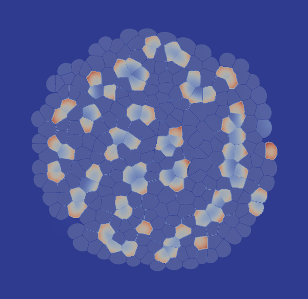
The following image gives you a foretaste of how the results of Turial 2 look like:

tutorial_02.png
t=10000: High receptor concentration is shown in red.